OpenPSN — the PSN neutron transport solver, in your browser

01Why a transport solver built on diffusion?

Deterministic neutron transport has always been a trade-off: diffusion codes are fast and simple but miss the physics near absorbers and in fine structure; discrete-ordinates codes (S_N/MOC) are accurate but expensive — and carry a permanent artefact, ray effects — fake dark corridors between tracked directions that never go away at fixed angular order. PSN resolves the trade-off: each node lives in space × angle, so the angular integral inside a node is continuous, and the node balance closes onto a standard diffusion equation.

Phase-space nodes

A PSN node is a spatial cell × polar segment × azimuthal segment. The angular flux inside is a P1 expansion in Ω·∇, whose φ₀ satisfies the standard diffusion equation — k² = 3Σ_t², angle-free. The node balance closes analytically; face currents are integrated in closed form.

ψ(𝐫,Ω) = ¼π⁻¹ [ φ(𝐫) − (1/3Σ_t) cosθ (n̂·∇)φ(𝐫) ] + C/4π

No ray effects

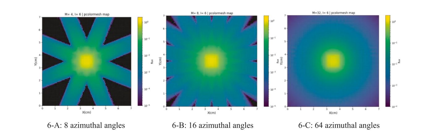
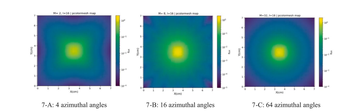
Directions are integrated continuously over each angular segment instead of being discretised into tracked directions. The classic MOC artefact — black corridors between tracks — simply cannot form. Verified against the paper's point-source problem: MOC shows rays at 8, 16, 64 azimuths; PSN is clean at 4.

∫ segment ψ(Ω) dΩ ⟶ closed form, no tracked directions

Fast by structure

With mirror boundaries the azimuth couples only m with M−1−m, so the global system block-diagonalises into I/2 × M/2 small dense systems. Coefficients are source-independent → LU-factored once; every power-iteration step is back-substitution. Convergence to 10⁻¹⁰ takes seconds in a browser tab.

A^(i,{m,m′}) u = b(q) → LU once, back-substitute per k-step

02The ray-effect test: same source, two solvers

A 1 cm source at the centre of a 7 cm scattering/absorbing box, vacuum boundary. MOC sees the source only through directions that happen to hit it — everything between the tracks goes dark. More azimuths fill the gaps, but the artefact is structural. PSN integrates the angular flux continuously, so the dark corridors never appear — not even at 4 azimuthal segments.

MOCArtificial ray effects persist

8 → 16 → 64 azimuths: dark corridors between tracks shrink but are never eliminated. The 64-azimuth MOC solution is still visibly striped.

Fig. 6 of Chao, Li & Chen (2027)

PSNNo rays, ever

4 → 16 → 64 azimuths: the PSN flux is smooth from the first column. At 4 azimuths it is already indistinguishable from the 64-azimuth result.

Fig. 7 of Chao, Li & Chen (2027)

PSN vs MOC convergence with space, azimuth, polar

Convergence to the Monte-Carlo reference as the grid refines — space × angle × angle

PSN vs MOC on the weak-absorber checkerboard: (A) spatial grid effect, (B) azimuthal-segment effect, (C) polar-line effect. PSN reaches the reference with far coarser angle discretisation — its convergence is limited by space, not by ray effects. The green dashed line is the converged 10×10 / 24-azimuth reference solution.

Fig. 1 of Chao, Li & Chen (2027)

03Run it — in this tab, right now

The canonical PSN checkerboard: a 2×2 unit-cell lattice of fuel (Σ_t=1.5, νΣ_f=0.24) and absorber cells, 1 cm base cells subdivided S×S, all boundaries mirror-reflective, one energy group. Pick a case and press Run — or grab a preset. The solver runs entirely on your machine; nothing is sent to a server.

psn.js — phase-space nodal solver, generic model (2.10), block-LU per mirror pair runs in your browser · no server · no dependencies

Absorber case

Subdivision S (S×S per cell)

Azimuthal segments M

k_eff tolerance

Result

k_eff

—

Δ vs OpenMC ref

—

Outer iterations

—

Wall time (this tab)

—

Convergence — |Δk_eff/k_eff| per outer iteration

log scale; green dashed line = target tolerance

Scalar flux φ (converged)

colour ∝ φ (global scale) white line = fuel ↔ absorber boundary

Brighter = higher flux: fuel quadrants peak bright, absorber quadrants are depressed. The white cross-marks delimit the fuel/absorber material blocks. Note the smooth, ray-free shape.

Solver log

ready — pick a case and press Run.

Polar lines (I/2)

Block systems / line

M/2

Block size (unknowns)

—

Nodes

Each (polar line, azimuthal mirror-pair) is an independent dense system whose coefficients do not depend on the source, so it is factorised once (LU) and every outer power-iteration step only back-substitutes. Same structural trick as the Python reference implementation.

04The published 60-point grid, reproduced

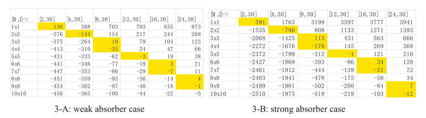
The complete eigenvalue grid of the paper's Sec. 4.1 (both checkerboard cases, S = 1–10, M = 2–24): our values, the printed values and the difference in pcm. The points inside the browser-solvable range were computed by this page's JavaScript engine — they turn green below the moment you run them above.

Diagonal valleys: PSN's space–angle correlation

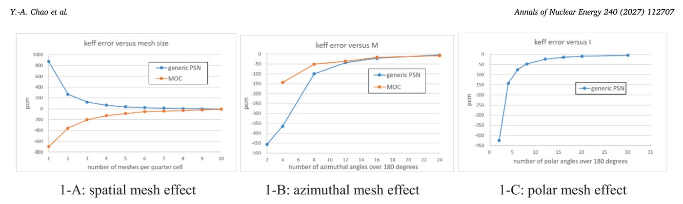
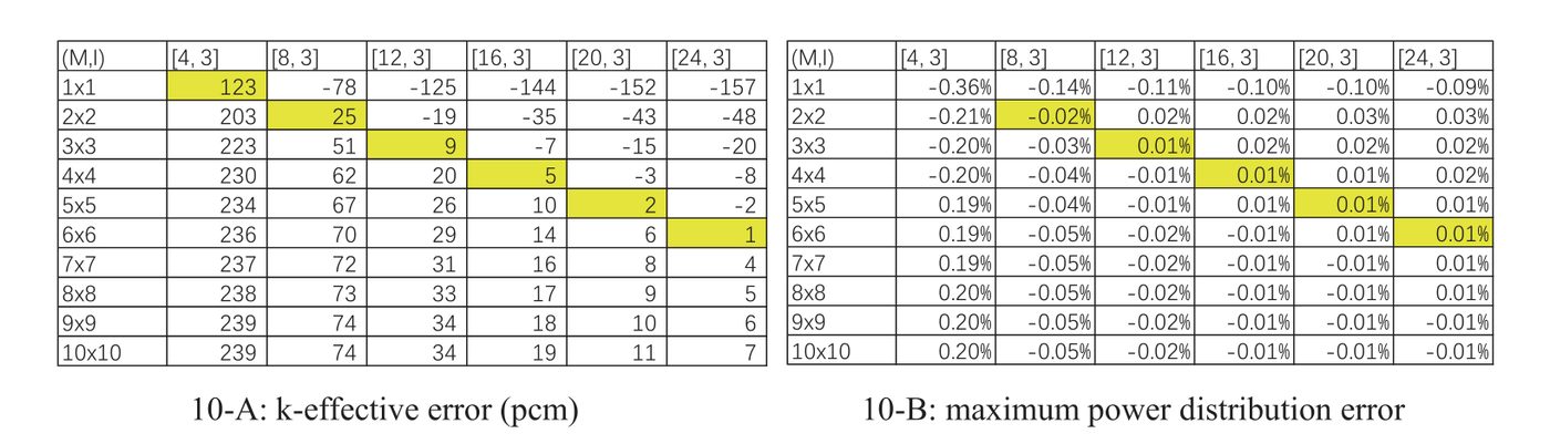
Look at the error heatmaps in Fig. 3 of the paper: the smallest errors don't sit in the bottom-right corner — they run along a diagonal. A 3×3 spatial grid with 12 azimuths matches a 10×10 grid with 24. The same correlation appears in the BWR bundle problem. We don't fully understand the mathematics yet — it is one of the most interesting open features of the method.

< 2 pcm

max |Δk_eff| across both 60-point grids
(Chao, Li & Chen 2027, Fig. 3)

S	M=2	M=4	M=8	M=12	M=16	M=24

Cell format: ours / paper (Δ), Δ = ours − paper in pcm; k_ref from OpenMC (Romano et al. 2015). Paper values as printed in Ref. [1], Figs. 3-A/B. Points outside the browser range (S ≥ 5) come from the Python reference implementation on a 48-core CPU and are identical to the paper's own appendix tables.

k_eff error (pcm) over the space × angle grid — the diagonal "valley" of near-optimal combinations

Left: weak absorber, right: strong absorber. Yellow highlight = closest-to-reference diagonal. The valley is where PSN gets transport accuracy from a fraction of the grid.

Fig. 3 of Chao, Li & Chen (2027)

05Beyond the toy problem

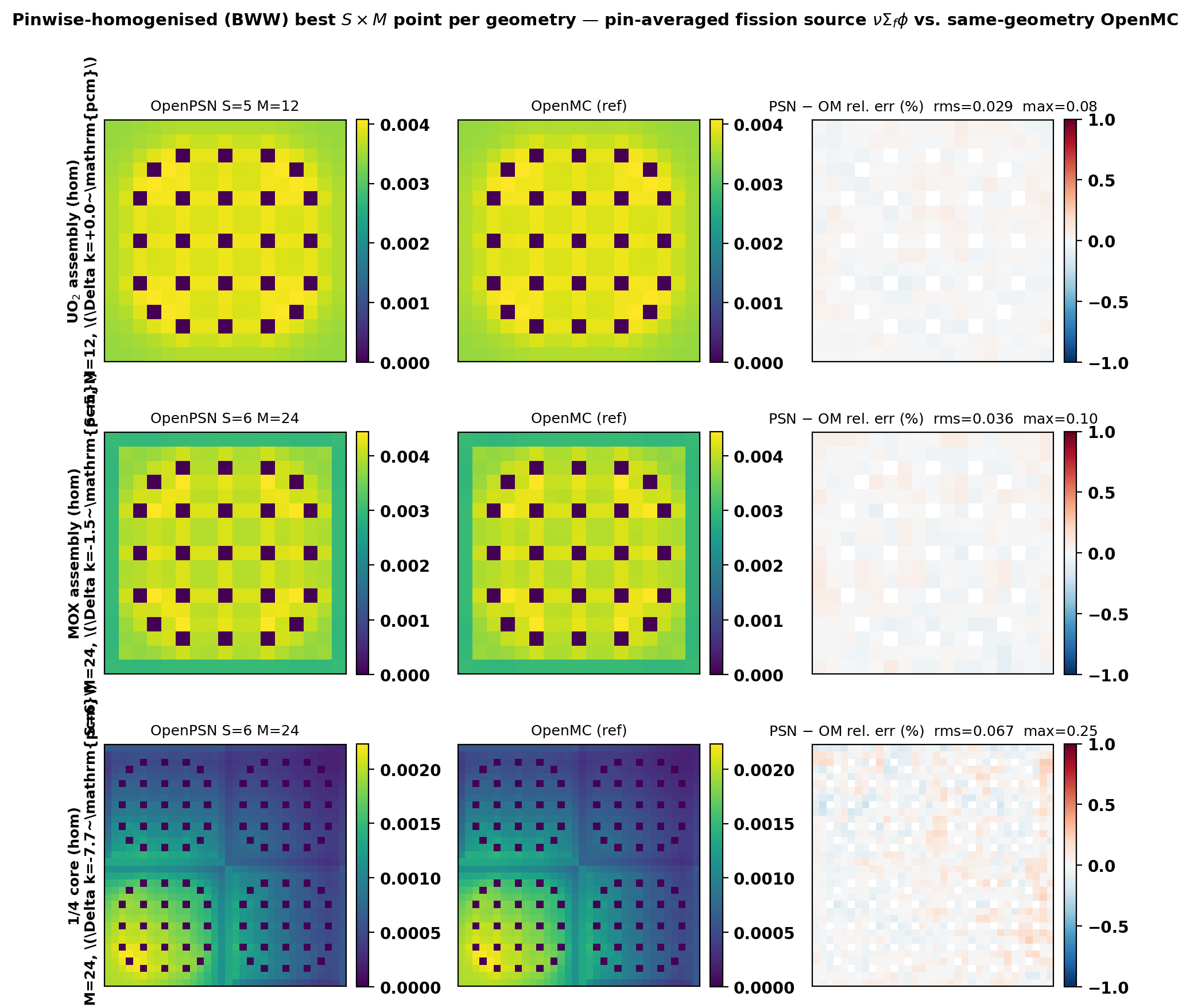
The browser runs the 1-group checkerboard. The full OpenPSN code (Python, multi-group, sparse) carries the same node model into real reactor problems.

C5G7 MOX 1/4 core, 7 energy groups — pin power and error vs reference

10404 nodes, 17×17 pin assemblies, 7-group C5G7 benchmark. Left: OpenPSN pin power; right: relative error vs the multi-group transport reference. The method's multi-group capability is exercised end to end — scattering between groups, pin-wise fission peaks, power shape.

OpenPSN preprint (2026), our computation

BWR 12-pin bundle, 2 groups

The paper's modified BWR assembly: with and without a Gd-bearing pin — the hard problem for any deterministic code (strong local absorption, two groups).

Fig. 8 of Chao, Li & Chen (2027)

BWR bundle, no Gd — PSN error over the space × angle grid

Top: k_eff error (pcm); bottom: max pin-power error (%). The diagonal valley returns: a 3×3 grid with 12 azimuths is as good as 10×10 with 24 in MOC.

Fig. 10 of Chao, Li & Chen (2027)

06How PSN works, in four moves

1 · The node: space × angle, closed in analytic form

In each phase-space node the angular flux is written as a P1 base function in Ω·∇. Its φ₀ solves the standard diffusion equation (k² = 3Σ_t², angle-free); face currents and face fluxes follow from closed-form angular integrals (β_i, α_f) — no quadrature, no tracked directions.

J_f = β_i(n̂ + cc·U)·(−1/3Σ_t ⟨∇φ⟩_face) Φ_f = α_f ⟨φ⟩_face

2 · The node map: 9×9, probed once

The map (J₄, q) → (Φ, φ̄, moments) is exactly linear in the 9 unknowns. It is probed once per (material, polar line, azimuth) with nine basis vectors into a 9×9 matrix — the vectorised trick behind the 107× speedup of the reference implementation.

[Φ(4), φ̄, m1x, m1y, m2x, m2y]ᵀ = S₉ₓ₉ · [J₄(4), q(5)]ᵀ

3 · The global system: small blocks, factored once

Interfacing all nodes gives a sparse system over face currents. Mirror boundaries couple azimuth m only with M−1−m, so the system block-diagonalises: 15 polar lines × M/2 mirror pairs independent dense blocks, each LU-factored once. Outer power-iteration steps are pure back-substitution — that is why this page converges in seconds on a laptop.

A^(i,{m,m′}) u = b(q) → LU once, back-substitute every k-iteration

4 · The eigenvalue: paraboloidal source, clean convergence

Standard power iteration with k-update, but the fission source keeps the full paraboloidal shape of the flux (q₀, q₁ₓ, q₁ᵧ, q₂ₓ, q₂ᵧ per node). Convergence criterion |Δk_eff/k_eff| < 10⁻¹⁰.

k_eff ← F_new/F_old · k_eff Q ∝ νΣ_f χ · (φ₀ + φ₁ₓP₁ + φ₁ᵧP₁ + φ₂ₓP₂ + φ₂ᵧP₂)

07References

Y. Xu — "OpenPSN: a multi-group Phase Space Nodal solver and its validation on the C5G7 MOX benchmark." Preprint, ResearchGate (2026). researchgate.net/publication/414038054. — this work: the C5G7-2D validation, code, and all results shown on this page.
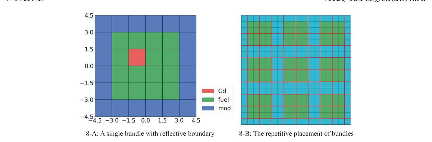
Y.-A. Chao, Z. Li, G. Chen — "Diffusion-based phase space nodal method (PSN): Solving the neutron transport equation with a diffusion code." Annals of Nuclear Energy 240 (2027) 112707. doi:10.1016/j.anucene.2026.112707. — the method; source of Figs. 3, 6, 7, 8, 10 shown on this page.
P. K. Romano, N. E. Horelik, B. R. Herman, A. G. Nelson, B. Forget, K. Smith — "OpenMC: A state-of-the-art Monte Carlo code for research and development." Annals of Nuclear Energy 82 (2015) 90–97. doi:10.1016/j.anucene.2014.07.048. — reference k_eff = 1.12974 (weak) / 0.51673 (strong) for the checkerboard.
H. H. Cho, J. Kang, J. I. Yoon, H. G. Joo — "Analysis of C5G7-TD benchmark with a multi-group pin homogenized SP3 code SPHINCS." Nuclear Engineering and Technology 53(5) (2021) 1403–1415. doi:10.1016/j.net.2020.11.013.
OECD/NEA — "Benchmark on Deterministic Transport Calculations Without Spatial Homogenisation: A 2-D/3-D MOX Fuel Assembly Benchmark," NEA/NSC/DOC(2003)16 (2003).
M. A. Smith, E. E. Lewis, B.-C. Na — "Benchmark on deterministic 2-D MOX fuel assembly transport calculations without spatial homogenization." Progress in Nuclear Energy 45 (2004) 107–118. doi:10.1016/j.pnueene.2004.09.003.
C. N. McGraw, M. L. Adams, W. D. Hawkins, M. P. Adams, T. Smith — "Accuracy of the linear discontinuous Galerkin method for reactor analyses with resolved fuel pins." PHYSOR 2014, Kyoto, 2014. — C5G7-2D resolved-pin reference k_eff = 1.186456.
W. Boyd, S. Shaner, L. Li, B. Forget, K. Smith — "The OpenMOC method of characteristics neutral particle transport code." Annals of Nuclear Energy 68 (2014) 43–52. doi:10.1016/j.anucene.2013.12.012.
G. Lathrop — "Effects of angular discretization in discrete-ordinates transport." Methods in Computational Physics 7 (1968). — the ray-effect problem PSN removes by construction.